Palettes
Palettes.RmdUnifrog Colors
This extracts the unifrog palette colours as hex codes. Examples below.
unifrog_colors()
#>       pink0       pink1       pink2        pink    darkpink     orange0
#>   "#feddef"   "#fcabd8"   "#fb85c6"   "#f95cb3"   "#be5787"   "#ffe4cc"
#>     orange1     orange2      orange  darkorange     yellow0     yellow1
#>   "#ffc999"   "#ffaf67"   "#ff7901"   "#af5d13"   "#fff2cc"   "#ffe699"
#>     yellow2      yellow  darkyellow      green0      green1      green2
#>   "#ffd966"   "#ffc000"   "#d88300"   "#cdf3e6"   "#adebd6"   "#85e0c2"
#>       green   darkgreen       teal0       teal1       teal2        teal
#>   "#33cc99"   "#188f67"   "#c9f0ef"   "#b7e9e9"   "#93ddde"   "#4bc7c8"
#>    darkteal       blue0       blue1       blue2        blue    darkblue
#>   "#348b8b"   "#dae9f6"   "#bdd7ee"   "#9dc3e6"   "#5b9bd5"   "#167ad5"
#>     indigo0     indigo1     indigo2      indigo  darkindigo     purple0
#>   "#e8e9fe"   "#dbddfd"   "#bcbffc"   "#9ba0fb"   "#4f58fc"   "#ecdff5"
#>     purple1     purple2      purple  darkpurple  background neutralgrey
#>   "#ddc5ed"   "#cba7e3"   "#bd90dc"   "#9036d6"   "#Ffffff"   "#F9f9f9"
#>   lightgrey    darkgrey        main
#>   "#CCCCCC"   "#999999"   "#000000"
unifrog_colors("green", "teal", "darkgrey")
#> [1] "#33cc99" "#4bc7c8" "#999999"
unikn
You can view the palettes in a pretty way using the
unikn package
library(unikn)
#> Welcome to unikn (v1.0.0)!
#> demopal() demonstrates a color palette.
seecol(unifrog_colors(), main = "The entire Unifrog colour scheme")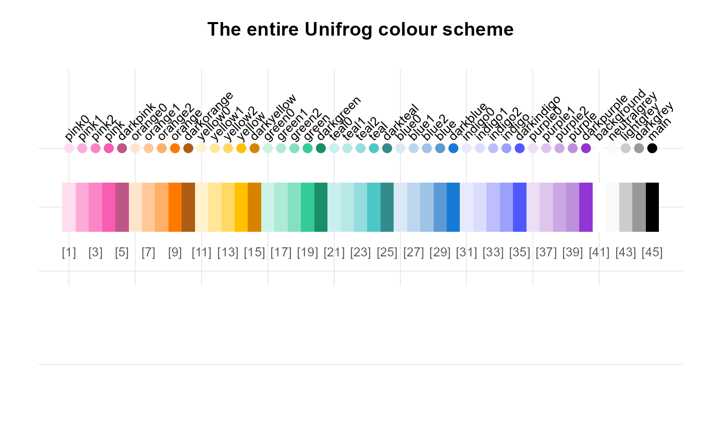
seecol(qual_vibrant, main = "The \"qual_vibrant\" palette is default for discrete data")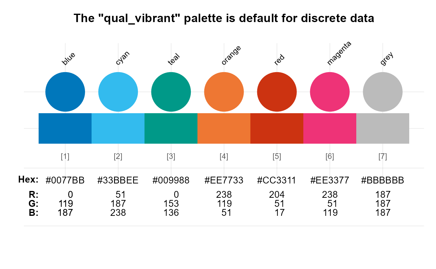
seecol(seq_iridescent, main = "The \"seq_iridescent\" palette is default for continuous data")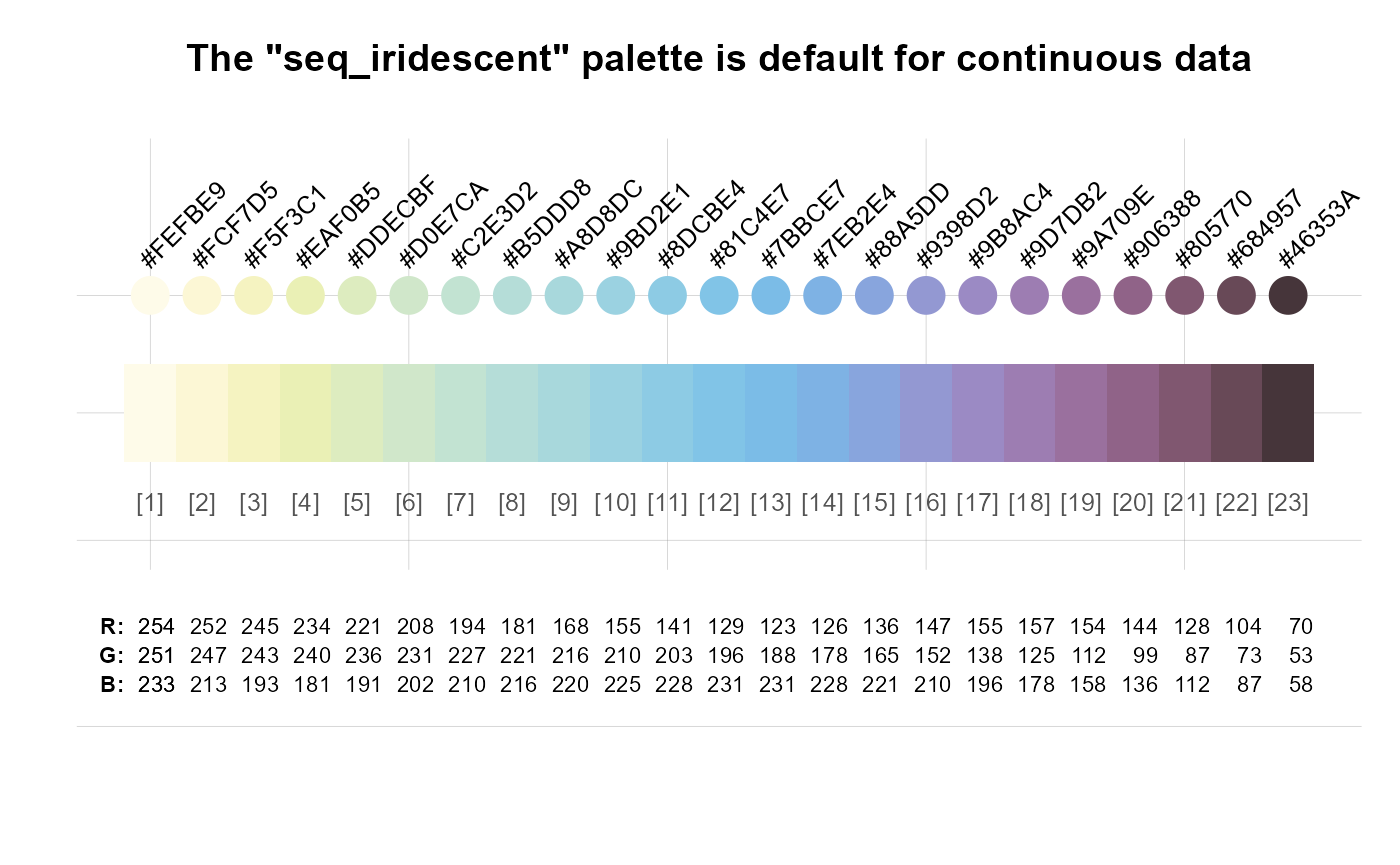
seecol(cb_palettes,
  main = "The names of all of the Unifrog palettes",
  pal_names = names(cb_palettes)
)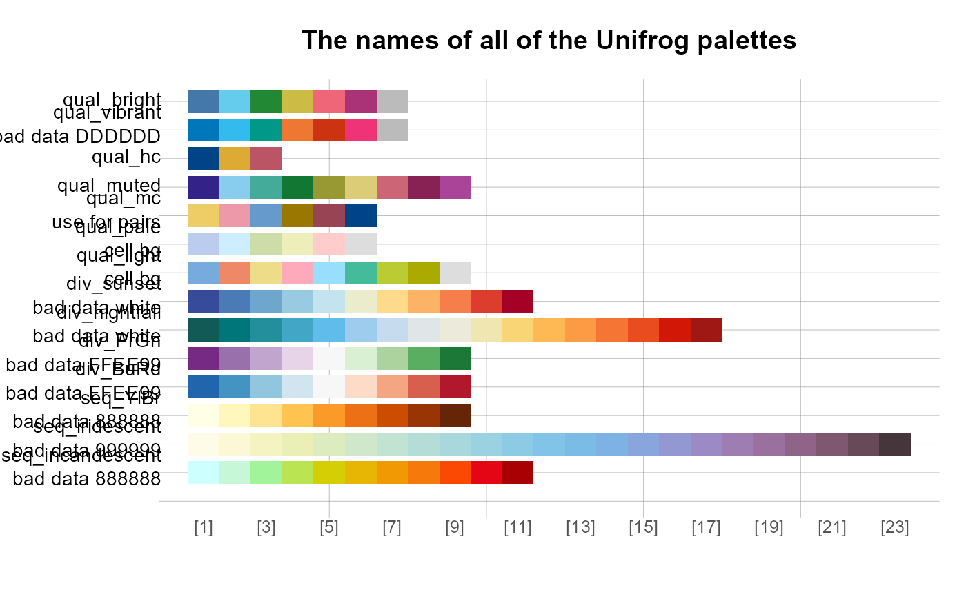
They have been grouped in three colour-blind friendly categories:
Discrete - ‘qual_bright’, ‘qual_vibrant’, ‘qual_hc’, ‘qual_muted’, ‘qual_mc’, ‘qual_pale’, ‘qual_light’
Sequential - ‘seq_YlBr’, ‘seq_iridescent’, ‘seq_incandescent’
Diverging - ‘div_sunset’, ‘div_nightfall’, ‘div_PrGn’, ‘div_BuRd’
scale_fill_unifrog
If no fill is specified, for a categorical variable, then the default
is scale_fill_unifrog_d("qual_vibrant").
ggplot(iris, aes(x = Species, y = Sepal.Length, fill = Species)) +
  geom_boxplot() +
  theme_classic()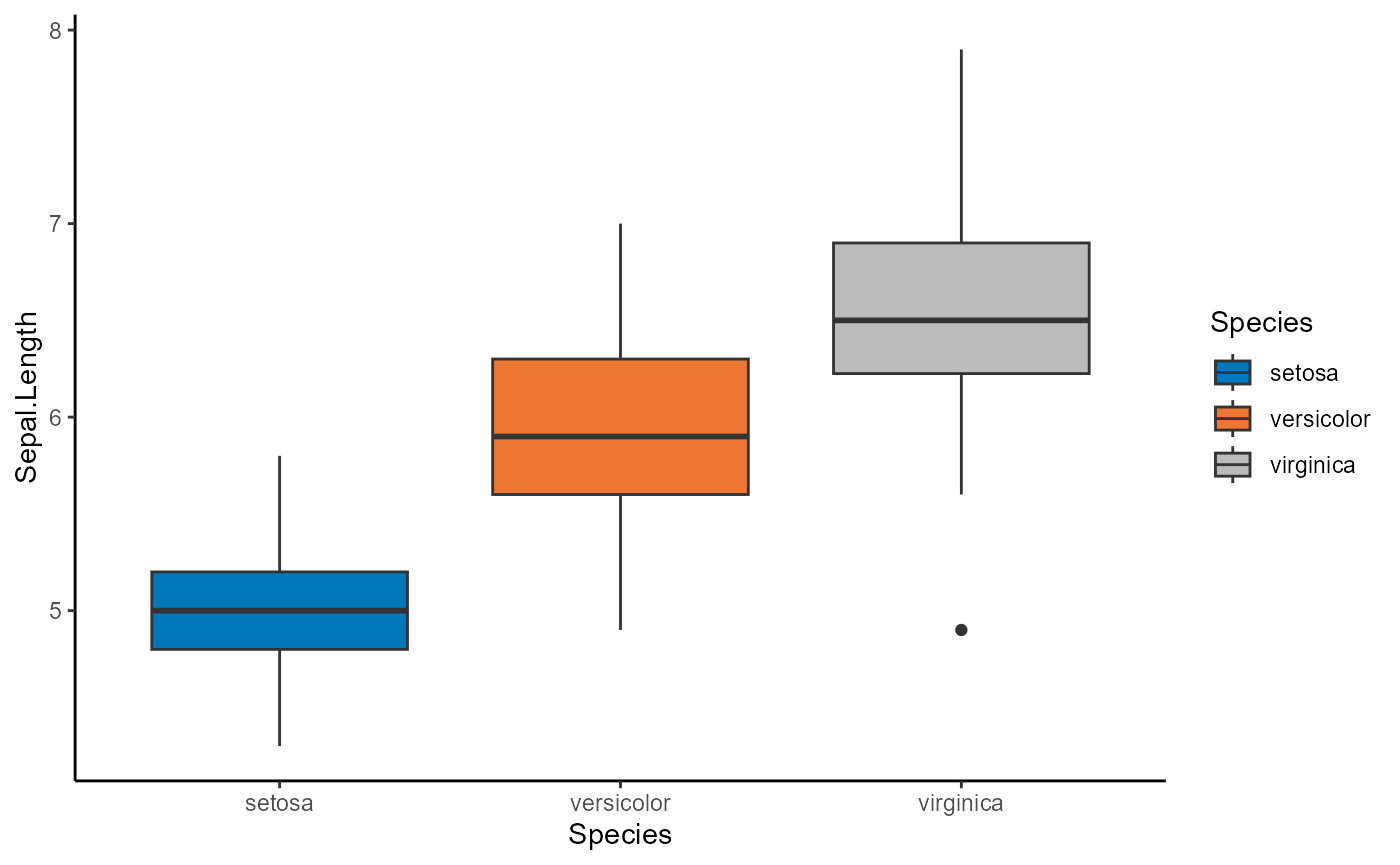
You can see that the addition of line 4 has no effect on the output
ggplot(iris, aes(x = Species, y = Sepal.Length, fill = Species)) +
  geom_boxplot() +
  theme_classic() +
  scale_fill_unifrog_d()
Addition of reverse = TRUE on line 4 starts from the
opposite end of the palette.
ggplot(iris, aes(x = Species, y = Sepal.Length, fill = Species)) +
  geom_boxplot() +
  theme_classic() +
  scale_fill_unifrog_d(reverse = TRUE)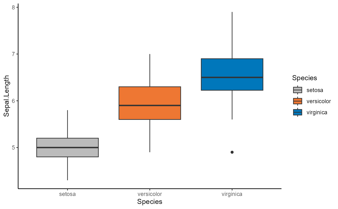
In order to guarantee the colour reversal for
qual_vibrant use fct_rev in the fill
argument.
ggplot(iris, aes(x = Species, y = Sepal.Length, fill = fct_rev(Species))) +
  geom_boxplot() +
  theme_classic() +
  scale_fill_unifrog_d()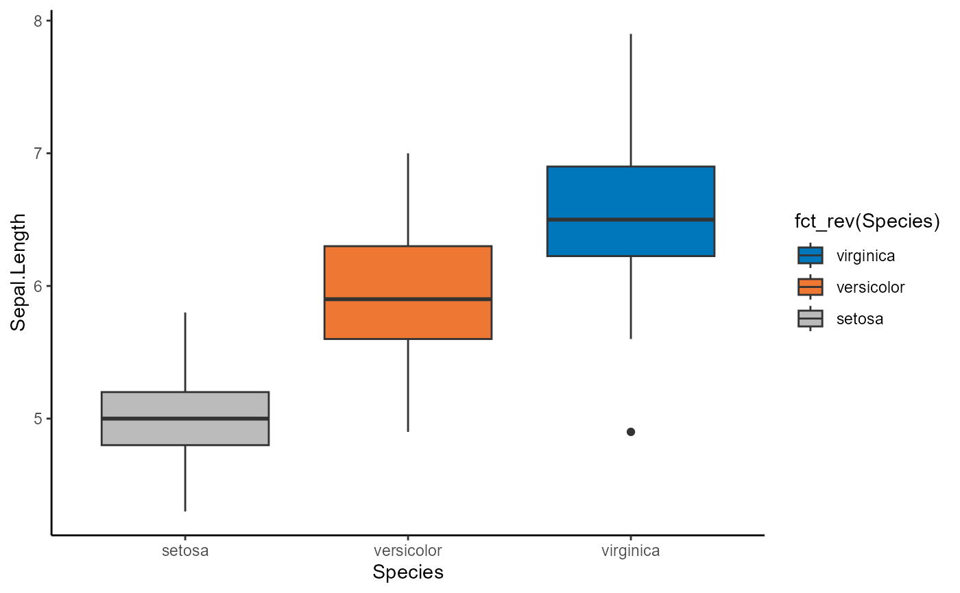
If you want to use a different palette, you can specify it with the palette argument.
Note a sequential palette does not often make sense for bar charts.
ggplot(iris, aes(x = Species, y = Sepal.Length, fill = Species)) +
  geom_violin() +
  scale_fill_unifrog_d(palette = "div_PrGn") +
  theme_classic()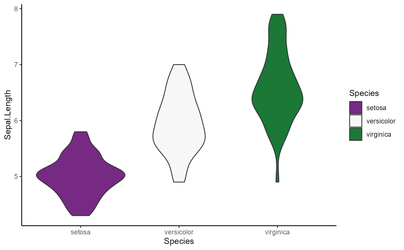
scale_color_unifrog
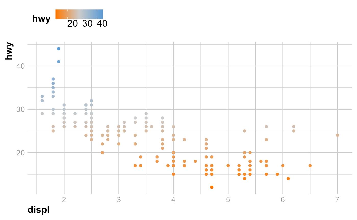
For continuous variables, the default is
scale_fill_unifrog_c("seq_iridescent")
ggplot(mpg, aes(x = displ, y = hwy, color = hwy)) +
  geom_point() +
  unifrog_theme(axis = TRUE)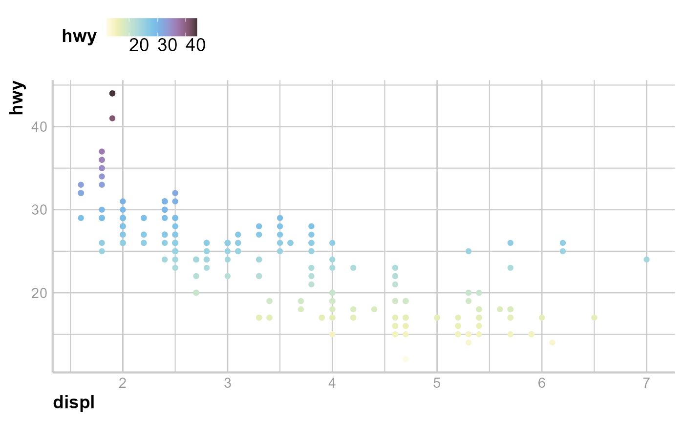
You can change this the same way as shown above but using the color aesthetic.
ggplot(mpg, aes(x = displ, y = hwy, color = hwy)) +
  geom_point() +
  scale_color_unifrog_c("likert3") +
  unifrog_theme()